

Structured logs

Naturally collected logs
Any application, be it large or small, benefits from collecting information about operations that occur inside of it, most commonly in the form of logs. Our platform is no exception and we too collect and store information about the happenings in the application for later review, analysis, or, in unfortunate scenarios debugging.
The most simple way of collecting and storing log information is a log file, in which every operation has its entry alongside some metadata (such as timestamps). Our platform goes a little further and stores the log entries in a separate MongoDB collection, so that it can be processed much more easily, than a text file.
The question is: can we do better? As you might have noticed we recently published a paper on our blog that goes deeper into this topic, you can give it a read HERE, if you are hungry for some more in-depth information. This post attempts to summarize the main point of the paper and to explain the basic concepts of our new structured logs in a way that is understandable, even if you are only testing the waters of the ocean that is Petri nets.
As you already know from our blog post about process-driven programming, the main advancement this paradigm has over traditional, more established, approaches, such as object-oriented programming, is that it defines a life cycle for its equivalent of classes – the processes.
Since the processes have an underlying structure given by the Petri net model it makes no sense to collect logs about them in an unstructured manner! Why should we have to wade through the marsh, that is the log entries, just to assemble the individual entries into a greater picture, if the application can do this for us in a more natural way!
Demonstration
Here comes the part, where we dive into the Petri net waters but fear not! We have pictures to help you follow our explanation! As you already know, Petri nets consist of transitions, places and arcs – explained HERE. Arc connections, along with the initial distribution of the tokens create dependencies between the transitions.
Let’s demonstrate this with an example. In the picture, you can see a simple net with three transitions and three places. Transitions A and B are independent of each other and can execute (fire) in any order. Transition C needs to consume two tokens from its input place however and can only be executed after both A and B were fired.
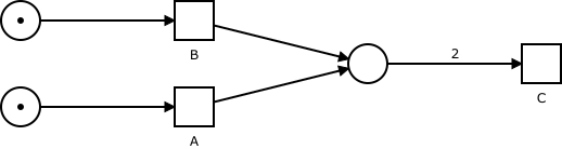
This creates an ordering of the possible ways the transitions in the net can be executed, but because not all transitions must be executed in a specific order (such as transitions A and B), this ordering is not complete. That’s why it is called a partial order!
We use this property of one transition depending on the firing of another to model processes and to express conditions and logical dependencies in our systems.
Let’s examine what would happen if we changed the net just slightly. The only change we have made to the net is we decreased the number of tokens transition C needs to consume from 2 to 1. This small change has altered the dependencies between the transitions and therefore also the behaviour modelled by this net.

In contrast with the previous example, where both A and B had to be fired, before C could fire, now firing either of them suffices for C to become enabled. Furthermore, once A or B was fired, C and the other transition can be fired independently of each other.
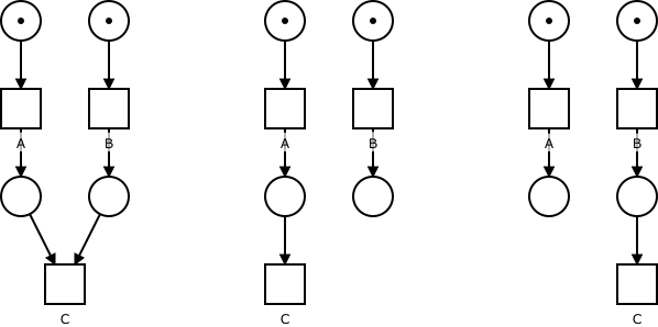
We can display the dependencies between transitions in a graph, and since, as we have just seen, they can differ from one instance to another each order of execution will have its own graph – its own run.
You can see the dependencies between the transitions, in all three runs described so far, in graph form on the picture below. These runs make the dependencies we have described earlier much easier to spot and, with more complex nets, can help us to spot design errors or perform some other analysis of the model. We could even use the captured runs as input for process mining procedures to create a model that would generate them.
One tool to rule them all
The new logging prototype module, we have developed does exactly this! Whenever a task in the application engine is finished, this information is added to the run graph of that case. Then you can use the search tools already present in our platform. Use them to filter only the cases and therefore their runs you are interested in. Afterwards, with a click of a single button, you can download all the runs of the selected cases and use them however you see fit!
But how would you open these graphs and examine them? Do you need a special tool to do it with? No! Our platform already has a way to represent graph structures – the Petri nets themselves! The new module takes advantage of this fact and generates and exports the runs in the same format, we use for our models – the Petriflow language. Because of this, you can use our existing tools – the application builder – to open and work with the generated data. But wouldn’t that make things confusing? you might ask. Well, judge for yourself! On the image below you can see the same runs expressed as Petri nets.
We hope this blog post shed some light on our paper or has motivated you to give it a read. Regardless, we hope to have entertained and/or intrigued you and we look forward to the many more exciting topics we have to discuss in our future posts.

Ready to modernize your business operations?
Try our Netgrif Application Builder and get your own Netgrif Platform experience.